Psychonomic History

Main Page

“Economic activities are inherently dissipative and governed by the second law of thermodynamics” – Robert Ayres

Introducing Thermodynamics

In this article, I hope to guide the reader and unearth a novel new way to think about the world, – psychonomic history and geopolitics included. In essence, an entropic view of reality will be discussed and by the end of the article, an entropic model that attempts to quantify a unipolar, bipolar and multipolar world scenario will be unraveled. The zeroth, first, second and third laws of thermodynamics are inviolable laws of the universe, they apply to everything – star systems, planets, ecosystems and societies. Entropy is an unspoken giant in our world – it is all around us, its laws are one of few truly inviolable laws of the Multiverse, yet entropy is easily misunderstood by most people. It will be my great honor to attempt to give the reader a deeper understanding of it, as an understanding of thermodynamics will greatly bolster the scaffolding of psychonomic history to its disciples. We need to understand some formal definitions first. The unapologetic march of thermodynamics has been the ruination of many empires led by madmen who have retreated to the illusions of permanent glory. Let us first cover some basic science to lay the groundwork. Thermodynamics is the study of energy, but its name imparts special meaning to heat in particular, and it will become clear why that is so. Energy is the potential to do work, but not all energy can be fully converted to work. Energy is defined in units of Joules. One Joule is equal to 1 Newton of force applied over a metric meter, 1J = 1Nm. Work (W) in physics has a very special meaning – it refers to an ordered form of energy that can be directed to do useful things like driving a piston in an engine. Therefore, work is a form of high quality energy: work is ordered, less random and has what is called, “low entropy”, compared to lower quality energy. But what is lower quality energy? There is heat (Q): heat is technically not a form of energy, merely a transfer of thermal energy. Think of thermal energy as the average vibration of particles.

The Laws Of Thermodynamics

The fundamental difference between work and heat (thermal energy) is that thermal energy is a far more granular “microstate” consisting of atomic vibrations proportional to temperature, while work is a more aggregated “macrostate” consisting of structures made up of atoms acting with force through a distance. This will become clearer later on. For the sake of generalization, we can say that heat is disordered, more random and has higher entropy than work. Energy with higher entropy such as thermal energy (vibration of atoms) is characterized by more randomness, it diffuses by naturally spreading out into its surroundings over time – heat is the most common mechanism of the transfer of thermal energy. The higher the temperature, the higher the thermal energy. Higher entropy forms of energy are less recoverable into useful work. Work and heat are related. You can convert 100% of work into heat but never 100% of heat into work. The disparity is why we cannot ever have 100% truly efficient machines or engines anywhere in the Multiverse. You can create 100% of order into disorder but not 100% of disorder into order. It is a fundamental principle of nature. Moreover, the mechanical equivalent of heat stipulates that if mechanical work is applied to say, a cup of water by swirling the water vigorously by some contraption, it will eventually raise its temperature exactly the same degree as an equivalent amount of heat transfer. Thus, work and heat can both raise the temperature of a system. This is where another well known unit of energy comes from, the Calorie. One Calorie is the amount of energy needed to raise the temperature of 1g of water at 15 degrees, by 1 degree Celsius. One Calorie is equivalent to 4.2 Joules of energy. The zeroth law of thermodynamics states that if 2 bodies are in thermal equilibrium with a third body, then they are also in thermal equilibrium with each other, despite not being in direct contact. The implications of this simple law are profound: if the third body is a thermometer, then the 2 bodies are in thermal equilibrium if they are the same temperature. Thus temperature becomes a proxy for measuring thermal energy of a system. A system is always defined by a boundary. Energy into and out of a system happens at the defined boundary. An adiabatic system is one where there is zero heat transfer (a perfectly insulated room) coming into or out of the room. If the room only contains an electric heater, the energy increase of the room is equal to the electric energy produced by the heater, since electric energy is a form of higher quality ordered energy, or work, 100% of it will be converted to thermal energy of the surrounding atoms in the room via heat transfer and no thermal energy can leak out of the room due to perfect insulation. In the real world however, thermal energy tends to “leak” out of the room to the surrounding environment.

Energy can take many forms and their relevance depends on the system being studied, most notably the level of granularity. Particles will have various quantum energies associated with vacuum fluctuations, spin and magnetism, plus rest mass energy. These forms of energy either find no counter-parts in macro systems or are treated as constants in the macro world. According to $E=mc^2$, the equivalence between energy and mass is mediated by the speed of light as the conversion factor between mass and energy. This may sound nonsensical at the human level, but it is very real and tangible at the quantum level where for example, nuclear fission is able to convert a small fraction of mass, which is an intrinsic form of energy, into its pure energy equivalent. A 64kg 90% enriched uranium core only needs 1.5% of mass to have fissioned into a chain reaction in order to detonate, but only 0.1% of the 1kg mass is converted into energy by the equation. That small amount of mass conversion into energy is enough for a thermonuclear explosion. For a macro system such as a car, its mass is treated as a constant and there is negligible mass-energy conversion. True 100% mass-energy conversion only happens between matter and anti-matter. The first law of thermodynamics states that energy is always conserved – it is never destroyed or created, it merely transforms state. Of course, all matter that exists in the Multiverse was at one point created at a hypothesized singularity event called the “Big Bang”. The reason why we exist is owed to a chance asymmetry between matter and anti-matter. Matter ever slightly dominated anti-matter in the Multiverse after the initial post-Big Bang plasma soup cooled down over hundreds of thousands of years, with sub-atomic particles coalescing to form macro “matter” due to the emergence of fundamental force fields. Prior to that, most sub-atomic anti-matter particles annihilated with most sub-atomic matter particles, forming pure energy in the form of photons of light. Freely moving sub-atomic particles do not constitute mass until they interact and coalesce around the Higgs field. Those that go on to form larger macro building blocks such as molecules or compounds form even larger masses such as black holes, stars and planets, with spacetime distorted by these masses, causing gravitational attraction. As the level of granularity scales up, relative entropy decreases and some information about the system is inevitably lost. Think of a asymptotic geometric series, at the microscale you may have an infinite series of terms that describe the system accurately, as you scale up you are forced to truncate the series to say, a few leading terms and some subleading terms. The tail of higher order terms you discarded away to approximate the total is the loss of information. Some forces become more or less active as we scale from sub-atomic particles to molecules, from molecules to dust, from dust to stars. Always bear this scaling concept in mind of micro-to-macro state and vice versa: it is paramount to understanding thermodynamics and entropy.

Gravity plays a very important role in large masses while quantum mechanics plays a very small role. On the flip-side, quantum mechanics plays a very important role in smaller masses while gravity’s effects are less pronounced, but it is thought that quantum gravity plays an important bridge between both worlds (not yet discovered). One day, a grand unification theory will discover the effects of quantum gravity and this will be a defining milestone in our understanding of the Multiverse, bridging the knowledge gap that currently exists between quantum mechanics, classical mechanics and relativistic physics. The light which permeated spacetime in our early Multiverse 380,000 years after the Big Bang singularity is the farthest, most distant light source that can ever be detected anywhere, therefore it is impossible to “see” what the Multiverse “looked” like less than 380,000 years after its formation. During the infancy stage, there were only pure sub-atomic particles (photons, quarks, electrons etc): atoms did not yet exist. Once residual sub-atomic particles coalesced into atoms, this allowed photons of light to finally stop scattering off plasma and travel throughout spacetime. Those early atoms went on to form all matter in the known Multiverse, including us, while the aforementioned early light became the oldest light in the Multiverse since the Big Bang, known as the Cosmic Microwave Background Radiation (CMBR). The state of a system is specified by two or more independent, measurable properties such as pressure and temperature for example. If those properties do not change, the state does not change and no energy is transferred – the system is in equilibrium. A path is a series of states a system passes through. Entropy is path-dependent, not an independent property of a system. How entropy changes depends on the path a system follows. An identical system converting work to heat versus one converting heat to work, will not have the same entropy. Only in the special case of a reversible process will they be equal, something that is largely an academic endeavour not found in the real world. A system can be an open or closed system. Most systems which are studied are assumed to be closed systems, delineated from their surroundings by boundaries.

The second law of thermodynamics states that there is an inherent direction to energy flow, giving rise to the arrow of time. Energy always spontaneously flows from high energy to low energy, with the reverse only possible with the application of work. A room spontaneously always becomes messier over time, unless one puts in effort to clean it. But the reduction in local entropy in the room through cleaning is offset by the global net increase in entropy by using electricity to power the vacuum cleaner, a process that releases thermal energy into the atmosphere at the powerplant. In any system, net entropy always increases (irreversible processes) or remains constant (reversible processes), it never decreases. The entropy generated by a system is allowed to be positive or negative. When this quantity is summed with the entropy change in its surroundings, the net difference must be ≥ 0. This is very important to understand. Uncertainty and statistics feed into the idea of entropy if we imagine disordered energy forms as having statistically higher uncertainty in predicting their positions or velocities. Temperature is a good proxy of energy levels, the second law can be thus interpreted as energy always spontaneously flowing from high to low temperature. Another version of the second law states that energy always flows from an ordered higher quality form to a disordered lower quality form. In other words, over time in the Multiverse, energy tends to spread out and diffuse into a form with less usefulness. Entropy can be regarded as the unavailability of energy in being harnessed for useful work. The law applies to cosmic phenomena as much as to human societies, and everything in between. According to the zeroth and first laws of thermodynamics, heat and work are indistinguishable forms of energy. But according to the second law of thermodynamics, they are very much distinguishable forms of energy. Finally, the third law of thermodynamics sets the lowest bound for entropy: at Absolute Zero, or -273 degrees Celsius, entropy is zero for a pure crystalline substance. This is the physically lowest possible temperature in the entire Multiverse. The nuance of pure crystalline substance distinguishes the statistical state of having only 1 possible configuration – there is nothing to distinguish a microstate from a macrostate – all atoms form one uniform state, they are identical and equally probable. A non-crystalline substance can have more than 1 state at Absolute Zero, therefore some uncertainty exists in its possible state.

A Heated Debate

A system does not have “heat” or “heat energy”. Thermal energy is the internal energy of a system caused by random fluctuations known as Brownian molecular motion. It is correct to say a system has thermal energy, as thermal energy is a state property depending on temperature, mass and volume. Heat is energy in transit due to temperature difference. A simple analogy would be water in a tank. The tank’s properties determine its internal energy: a large tank with good insulation would have higher internal energy capacity. Water in a full tank would be akin to its thermal energy. If a pipe is connected from the tank to a height and temperature differential, pressure would cause water to flow and water flowing through the pipe would be like heat transfer.

If the system being studied is a “cup of coffee”, then the boundary of the system will be delineated as an invisible cutout around the cup of coffee with its surrounding environment. All energy flows across the boundary will affect the entropy of the system. Everything around the cup – the table on which it rests, the room within which it is located and the outside environment which envelops the dwelling hosting the room etc, can be considered as the “external environment”. So if the cup of coffee generates positive entropy, when summed with the entropy change in its surroundings, the net difference must always be ≥ 0. If somebody pours hot coffee into a cup at 100 degrees Celsius and places the cup on the table, what is happening to the entropy of the cup? If left to its own devices i.e. a spontaneous process, at an atomic level (micro level) the atoms are vibrating and transferring thermal energy to their neighbours in a chain reaction away from the hot source, from higher to lower temperature. The atoms in the surroundings are recipients of this cascade of energy transfers until equilibrium is reached between the cup of coffee and the room when both temperatures equalize. By that stage, the thermal energy has mostly dissipated out of the cup of coffee and into the room and outside the room via a mix of conduction (direct contact with the table), convection (heat fumes) and radiation (invisible to the naked eye). The spontaneous dissipation of thermal energy away from the hot source reduces the entropy of the cup, since the end state of the atoms in the coffee slow down and vibrate less vigorously than their initial state. There is less chaotic motion to their available configurations but more possible states available to the atoms to occupy as they consolidate towards more uniformity.

This is why 1 Joule of energy applied to a cold cup increases entropy more than a hot cup. As the cup cools down, it has less entropy than before – this is the local decrease in entropy but it does not violate the second law of thermodynamics. While the cup is in equilibrium with the room and its surroundings, there is an entropy increase in the external environment where the excess thermal energy has dissipated to. That entropy increase must be at least equal to, if not more, than the entropy decrease in the cup. The energy lost through cooling down is no longer available for useful work, this is what a net increase in entropy signifies – irreversible losses. The rare exception of reversible processes where the net entropy change in the entire system is zero, is largely academic. In the real world, most processes are irreversible due to energy being lost to entropy that can never be recovered back to useful work, making reversible harnessing of energy impossible. If instead, somebody pours hot coffee into a cup at 100 degrees Celsius and places the cup on the table then proceeds to stir the coffee vigorously while it is cooling down, through the mechanical equivalent of heat the application of work in stirring offsets cooling, making it possible to hold the temperature steady or even raising the temperature of the cup. Correspondingly, the entropy of the system moves in the opposite direction, even increasing, so long as the work done is vigorous enough to offset the cooling effect. The moment work ceases and the cup is left on its own, spontaneous entropy decline in the cup proceeds as usual (while still increasing overall in the external environment). This is how entropy can locally decrease while increasing globally in accordance with the second law of thermodynamics. The nuance depends on how the system is framed and defined. At the boundary of the cup and the immediate air above it, there is a temperature gradient between the temperature of the hot and cold source. This is the temperature gradient where integration happens in the entropy equations.

The Importance Of Scaling

For a process to occur, it must satisfy the first and second laws of thermodynamics. At this point, the reader may be pondering how exactly to define the boundary between a “microstate”, or “micro” system, and a “macrostate”, or “macro” system. There is no formal definition, the distinction is fairly arbitrary although several conditions are noteworthy:

• “Micro” level often corresponds to sub-atomic particles (photons, electrons, quarks) or atoms where quantum effects dominate: superposition, entanglement, spin, coherence or tunneling. The system can be better modelled with a discrete framework rather than a continuum framework. This is a realm where the system scale is on par with its own size, in wavelength. When a photon and an electron interact for example, if the energy of the single photon is on par with the energy packet required to excite a single electron up or down an allowable quantum (discrete) level within an atom’s orbital, the system is likely a “microstate”. According to the wave-particle duality, every wave and particle with a mass moving at a velocity (momentum) has a corresponding wavelength no matter its size, known as a de Broglie wavelength, given by the Planck constant (h) divided by its momentum (p): ($λ_{dB} = h / p$). At relativistic speeds (speeds approaching the speed of light), the de Broglie wavelength is stretched by the Lorentz factor to equal its Compton wavelength. Quantum states are unique in that there is an inter-dependence on the measurement among
  its observable and non-observable properties, the act of measuring those properties affects the system’s state (we will get into that shortly). A photon’s own wavelength is on scale with its own size compared to the wavelength of say, a truck, which would be negligible relative to its size. As such, quantum particles are affected by their own wavelengths in spacetime and those of neighboring particles, – this phenomenon alters their geometries and configuration state space. If quantum coherence is well maintained in a given system, there is an interdependence on the measurement among its observable and non-observable properties such as entanglement, superposition and spin. But “microstates” can also be metaphorical and not necessarily restricted to the quantum level. If analyzing a geopolitical system, the “microstate” equivalent would be a state defined by the most granular entity within the framework, such as an individual country.
• “Macro” level often corresponds to collectives of “micro” particles where quantum effects tend to be negligible. As the system grows towards a large number of particles N, it can be better modelled with statistical mechanics and behaves with averaged quantities. Classical physics is better suited in analyzing such a system with “macro” averaged properties such as temperature, pressure, volume and force. This is a realm where the system scale is not on par with its own wavelengths. If quantum coherence is not well maintained (i.e. quantum decoherence) and is easily broken, the system shows fragility where quantum coherence effects are unstable and easily erased by interference with neighbors. Granular information in this context is lost, suggesting a “zooming out” effect towards a more macro perspective. As such, entropy always decreases as scale moves towards a more aggregated form, resulting in some information loss with bulk behavior – we are no longer able to describe the system with granular properties reserved for microstates.
• There exists a scale that straddles between “micro” and “macro”, the mesoscopic realm. Here both quantum and classical physics affect measurable properties. Nano-technology, nano-materials, condensed matter physics and cryogenics (superconductivity) often straddle the mesoscopic realm.

Lower Limits

It is worth exploring in more detail, the lower limit as to how granular we can continue to “zoom into” reality. Apart from Absolute Zero (-273 degrees Celsius) in the temperature scale forming a minimal temperature floor in the Multiverse, Planck length and Planck time represents the smallest possible units of space and time that can be physically measured. However, measurements on par with these magnitudes are not only bounded by scale but also by the standard deviation (uncertainty) in their actual measurements. The act of measurement at these scales affects the state being measured in ways that we do not experience in the non-quantum world. The way the Planck length and time were derived is fascinating in itself. The units were derived purely from dimensional analysis using other constants of nature. The Planck length is given by taking the square root of the ratio of the multiplicative of the gravitational constant G and modified Planck constant ℏ with the speed of light cubed: √(G⋅ℏ/$c^3$) ~ 1.616×$10^{-35}$m. The Planck time is given by taking the square root of the ratio of the multiplicative of the gravitational constant G and modified Planck constant ℏ with the speed of light raised to the power of 5: √(G⋅ℏ/$c^5$) ~ 5.391×$10^{-44}$s. The values set the lowest resolution limits in space and time, below which we do not understand how reality behaves. Reality on these scales is governed by quantum mechanics but our picture of reality is still incomplete and it is thought that quantum gravity exerts noticeable effects on reality at these scales. Quantum gravity is a hypothesized unified physics between quantum mechanics and gravity, where both currently irreconcilable forces are thought to interact with each other in fundamental ways.

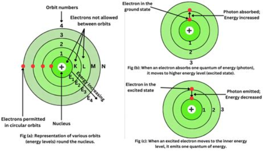
Max Planck was a German physicist who derived another fundamental constant in nature – the Planck constant (h), which comes out to be h = 6.626×$10^{-34}$J⋅s in units of energy over unit time. At its essence, the Planck constant represents the smallest discrete amount of energy that can be exchanged across time in all of space. At the Planck scale of quantum mechanics and quantum gravity, energy is no longer continuous as we perceive in the macro world. The finest grain of reality is discrete, where only discrete packets of energy are allowed to be exchanged in nature among the fundamental particles. Fundamental particles such as photons, electrons and quarks exchange energies in discrete amounts and can only jump between levels in accordance to discrete steps or quanta, i.e. Planck units of energy. The famous equation E = n(h⋅f) represents the energy of a photon which is proportional to the Planck constant h and the frequency of the energy source. High frequencies are thus associated with higher energies imparted to their photons. Note how only whole integer steps, or quanta n, of energies are allowed. This is the discretized nature of energy at the Planck scale. There can be no energy a photon is permitted to possess that exists between two quanta of energies. Likewise, an electron is simply unlikely to be found in certain regions around a nucleus where destructive interferences cancel out – these are the regions between quanta of energy levels. The probability of finding the particle there is modelled as very low.

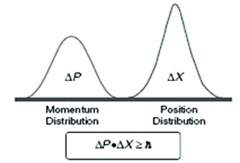
Finally, we come to the inevitable: the Heisenberg Uncertainty Principle. You cannot both have 100% accuracy in position or momentum: there is a real, measurable tradeoff between the two. If you wish to know a particle’s position in the wave more accurately, it comes at the cost of measuring its motion and momentum with less certainty. The opposite is also true: if you wish to know a particle’s momentum accurately, you will have greater uncertainty in its position. The principle goes to show a lower bound between the multiplicative of both quantities of standard deviation: σ$_x$⋅σ$_p$≥ ℏ/2 as more certainty is known about position, σ${}_x$ falls and σ${}_p$ in momentum must rise to compensate and keep the minimum energy allowable. The Multiverse does not allow precision at the quantum level for both position and velocity. The act of measurement disturbs the state of the system being measured, and the level of uncertainty in the measured quantities being disturbed are captured in a lower bound by the Uncertainty Principle.

To describe a particle’s state in space and time, there exists a time-dependent Wavefunction, ψ(x,t​). This equation describes how energy evolves over time, split into a kinetic and potential energy component for the particle. When solving higher order equations such as partial differential equations (PDEs) their solution is not a number but a function. In reality, the Wavefunction is an unknown physical object, and wavelets are used to model and approximate its behavior especially particle behavior, which are localized Gaussian curves which mimic wave packets in time and space. The solution to the Wavefunction is the Schrodinger function which takes several forms. One is the time-dependent solution, which describes in time how a particle evolves in accordance to the conservation of energy, where its state is proportional to its energy sum total at a given time. The probability distribution for finding a quantum particle is given by the Born Rule, which computes the square of the magnitude of the function, ∣ψ(x,t)∣$^2$. A function with higher magnitude has a higher probability of being in that state, just as vectors with longer lengths correspond to higher magnitudes, this is how probability is modelled at the quantum level, by using statistical distributions and probabilities. It goes against the deterministic nature of classical mechanics. Quantum particles are modelled by probability functions and probability clouds. During the early 20th century, this revolutionary concept of indeterminism threw out old notions of a deterministic Multiverse.

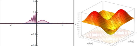
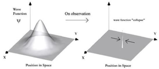
The time-independent solution on the other hand, is a special case of stationary standing waves for a particle. Standing waves are a special type of constrained wave, imagine a Saz string being plucked by a musician. The string is fixed at both ends, only certain quanta of notes are allowed in the harmonics of the fundamental frequency note. This is a standing wave. In a similar vein, an electron’s orbit around a nuclei is constrained by certain standing waves which are allowed, in quanta n of a fundamental frequency f i.e. n⋅f. Regions where the standing waves interfere constructively, the electron is allowed to orbit: regions where its standing waves destructively interfere, the electron is not allowed to orbit. The particle is never stationary per se, only the measurable shape of its probability density is frozen in time, given by ∣ψ(x)∣$^2$ without time. What motion must it possess to give a probabilistic stationary state? It must generate a zero entropy rate over time, since the probability density is fully predictable over time. But its state over space is unpredictable, so its entropy rate in space is positive. The sum total of its temporal and spatial components in entropy are changing at an extremely fast pace each nanosecond. Sometimes they may give a positive or a negative entropy, but the net entropy effect summed with the surroundings must always be ≥ 0. A particle’s total energy must be conserved at any given time, and its state is governed by the interplay between its kinetic and potential energies, which form standing waves and interfere with each other in space. This is why a particle’s behavior is difficult to model and quantum mechanics shows higher randomness and positive entropy generation than macrosystems where kinetic and potential energies do not interfere with each other in measurable ways and macrosystems are able to form more deterministic and orderly arrangements. In simple terms, there are more statistical combinations of configuration states with deeper inter-dependencies between time and space so energy tends to disperse more. One of the prominent solution forms to both Wavefunctions is a Gaussian curve, able to form narrow peaks localized in space, but also controls for flatter peaks, an ideal fit for the Uncertainty Principle. Since the total energy of a particle is the sum of its kinetic and potential components and must be conserved at all time, if the kinetic component rises, the particle has higher momentum. If we wish to measure momentum, the act of measurement forces the superposition of wave states to collapse and the momentum spread narrows at the expense of its potential energy spread, which widens. Position uncertainty and entropy increases. If you wish to know more accurate position information, the reverse happens. The act of measurement forces the superposition of wave states to collapse and the position spread narrows at the expense of its kinetic energy (momentum) spread, which widens. Momentum uncertainty and entropy increases.

Upper Limits

At the upper limits, Relativity and the invariant speed of light become very important limits. There are very few laws of nature that hold absolutely across the Multiverse, the laws of thermodynamics are one such set, the other is the absolute speed of light, which forms a maximum upper bound to any information exchange allowed anywhere in the Multiverse. To understand how the speed of light was derived, we need to discuss photons, the fundamental carrier particles of light and all electromagnetic radiation in the Multiverse. Photons are a special particle, they are never found at rest in nature nor can they ever be brought to rest, as they are considered massless and have zero rest mass. There are no stationary photons and no slow moving photons in spacetime. All photons travel at the exact speed of light, all the time, and everywhere. This has significant implications for the theory of Relativity and the speed of light. The theory of Relativity has two subsets: the Special Theory of Relativity (constant speed, zero acceleration) and the General Theory of Relativity (accelerated systems). The theory in general asserts that simultaneous events are not really simultaneous, they depend on the reference frame of the observers, i.e. simultaneity is relative, not absolute. Each observer is in a reference frame relative to the object being measured, and will measure different quantities from another observer in a separate reference frame. The reference frame could be at the same speed as the object, rendering the object relatively stationary to the observer. The observer could also be stationary relative to a moving object, rendering the object relatively moving to the observer. These notions form the backbone to Relativity.

For a photon, no such rest inertial frame exists. This has profound consequences. As such, all observers measuring photons will measure the same exact invariant speed regardless of their own reference frame. The empirical justification to the absolute speed of light traces back to the days of James Maxwell, a brilliant Scottish physicist who unified electric and magnetic forces into ‘electromagnetism’ – a fundamental force and field that permeates the Multiverse alongside other fundamental fields such as the Higgs, quantum and gravitational fields. The Higgs field for example, is a field that permeates all spacetime, assigning a non-zero value at every point in the vacuum of spacetime. When an object moves through the field, its coupling with the field causes “mass” to manifest as the equal and opposite force, a resistance against any energy change. We call this “inertia” or rest mass. Larger objects moving through the Higgs field gain more “mass”. Photons however, have zero mass because they do not interact with the Higgs field in any way. This is a fundamental property of the Multiverse. Maxwell made the discovery that a change, or flux, in an electric field causes magnetism and a flux in a magnetic field causes electricity. Static fields do not cause magnetism or electric current, only changes in fields do. This is why solenoids are always in motion. Maxwell encapsulated his unification of electric and magentic fields into 4 elegant equations dubbed Maxwell’s Equations. One of the equations, Faraday’s Law of Induction, states that the circulation density of an electric current is proportional to the rate of change of magnetic field over time.

Having discovered that magnetic and electric fields are inextricably linked in nature, he went on to estimate their speed. Maxwell took another 2 fundamental constants in nature, the electric permittivity of vacuum (how electric fields respond to electric charges), $ε_{0}$ = 8.854×$10^{-12}$ F⋅m$^{-1}$ and the magnetic permeability of vacuum (how magentic fields respond to electric currents), $μ_0$ = 1.256×$10^{-6}$ N⋅A$^{-2}$. He then calculated the speed of an electromagnetic wave as c$^2$ = 1/(ε$_0$⋅μ$_0$), giving the exact speed of light as c = 299 792 458m⋅s$^{-1}$. It is extraordinary that every single photon in the Multiverse travels at this exact speed, not faster, not slower, no matter the frame of the observer. Light is thus a disturbance in the electromagnetic field, and all carriers of light and radiation throughout the Multiverse, photons, move exactly at the same speed forever, they are never stationary and have zero mass. This is what allows them to travel at the speed of light with zero coupling to the Higgs field imparting them with no inertia. Photons are a self sustaining oscillation of the fabric of spacetime, where both electric and magnetic fields act orthogonal to each other and to the direction of motion. No work is done on the photon, the oscillations of the fields sustain each other – when the magnetic field is a maximum, electric field is a minimum and vice versa. This gives rise to the constant self-propagating nature of light. The source of a photon determines its energy and frequency (wavelength) – they can originate from gamma ray bursts, black holes, fires or radios. But the source does not determine their speed. This is a constant set by spacetime, a fundamental property of the Multiverse. When Albert Einstein developed the theory of Relativity, he found that in order to honor the invariant speed of light throughout the entire Multiverse, i.e. having no rest reference frame of its own, distance and time had to “bend” to satisfy the constant. It was a revolutionary insight totally at odds with the established thinking at the time.

It is why relativistic effects are felt only at relativistic speeds near the speed of light. Einstein merely modified Newtonian equations of motion with a correction factor to account for high speeds. Regular classical mechanics equations require a dimensionless correction factor to account for the expansion or contraction of length and time due to relativistic speeds, called a Lorentz factor γ = √(1 – v$^2$/c$^2$). The correction factor scales quantities of length and time when they travel at high speeds (v) nearing the speed of light (c). Concepts such as time dilation and the twins paradox arise from Relativity. When speeds are non-relativistic (very low), the Lorentz factor equates to 1 and becomes irrelevant. Objects that travel near light speed are measured from a relative frame of reference as slowing down in time (their clocks tick slower) and contracting in length. The objects themselves do not experience any such changes, it is merely relative. If a twin travelled near the speed of light at 99.944% the speed of light, the Lorentz factor would be 30. For their twin on the Earth frame, the trip would take 60 years while for the twin in the moving frame, the trip would be contracted to only 60/30 = 2 years. For both reference frames, the conserved quantity is distance squared Δs$^2$=(cΔt)$^2$−(Δx)$^2$−(Δy)$^2$−(Δz)$^2$ which can be thought of as a Pythagorean “equivalent” of spacetime with one term representing the temporal dimension and 3 terms each representing the spatial dimensions. However, unlike Euclidean space, the triangle inequality does not hold and the quantity is not always positive. The temporal and spatial components are subtracted from each other to accommodate for the Lorentz factor so that one reference frame sees more time and less space while another sees less time and more space, yet both agree on and compute the same conserved quantity Δs$^2$. In the example above, if we assume 1 dimension (x) we get Δs$^2$=(cΔt)$^2$−(Δx)$^2$. For the twin on the Earth reference frame, the time separation is Δt = 60 light years while the spatial separation is Δx = v⋅Δt = 0.99944c×60, giving Δs$^2$=(cΔt)$^2$−(Δx)$^2$ = 3600c$^2$ – 3596c$^2$ ~ 4 light years$^2$. For the twin on the moving reference frame, the time separation is Δt = 60/30 = 2 light years while the spatial separation is Δx = 0, giving Δs$^2$=(cΔt)$^2$−(Δx)$^2$ = 4c$^2$-0 ~ 4 light years$^2$. Each observer sees a different amount of time vs space but their total quantity is always conserved and equal. Space and time are thus intertwined into spacetime to keep the speed of light invariant. Mass and energy are also intertwined into mass-energy (E = mc$^2$) through the speed of light, causing space to bend and distort. These distortions and curvatures in spacetime due to mass-energy is what gives rise to gravity. Gravity is the curvature of spacetime and the tendency for mass-energy to accelerate within it.

Energy

Let us focus on phenomena that exists between the lower and upper limits of reality, i.e. non-relativistic speeds and a macrosystem level of grain. A unit of energy is known as a Joule (J), which is the application of 1 Newton (N) of force across 1 meter in 1 second. In turn, 1N of force is the force needed to move 1kg across 1 meter in 1 second. Therefore 1J = 1 kg⋅m$^2$⋅s$^{-2}$. The total energy (E) of a macro system above sea level is generalized to be the sum of its internal energy (U), kinetic energy (KE) and potential energy (PE). In equation form, the delta symbol (Δ) represents a change between an initial and final value across a two different states over a finite time, with the initial value subtracted from the final value. The total energy change is given by:

ΔE = ΔU + ΔKE + ΔPE (Equation 1)

where U = m×C$_{av}$×T, KE = 0.5×m×v$^2$ and PE = m×g×h, for a given mass m at temperature T, velocity v, height h above ground, average specific heat capacity C$_{av}$ and gravitational acceleration is g (9.8m/s$^2$) on the Earth’s surface.

Thermodynamics is not so much concerned with absolute values of energy like the value of KE or E at any given state. Like many properties in physics, changes in properties are more important than absolute values of properties. Changes in energy highlight the direction of a system’s evolution. Net entropy can be zero or positive, but never negative: it is always increasing with time or at best static. The change in entropy between 2 states is more valuable than absolute values of entropy on their own. An initial state can even be assigned an entropy of 0 so that its final state can be computed and compared to the initial value. The internal dynamics and shifts between energy forms in a system is key to understanding how entropy evolves within a system. For example, looking at the equation KE = 0.5×m×v${}^2$, kinetic energy is proportional to the square of the velocity (KE quadruples when velocity doubles) and linearly proportional to mass. Potential energy is proportional to the vertical height away from gravity. Internal energy is proportional to metabolic chemical energy and thermal energy (temperature). A stationary system has zero changes in KE and PE: all energy dynamics are internal – for example a bar being heated over time. In the case of a non-stationary system, a ball is thrown up into the air from the ground. It commences with maximum kinetic energy after being thrown, reaches a maximum height where kinetic energy reaches a minimum (zero) while potential energy reaches a maximum, then reverses: as it falls, potential energy exhausts to a minimum (zero) as it hits the ground while its kinetic energy is at maximum the moment before impact. A reversible process is one that can go in both directions without leaving any trace on its surroundings. Entropy for a reversible process is at best conserved (constant), i.e. the net change on the Multiverse is zero. Since we cannot get any better than a reversible process, we can never have a net negative entropy process in the Multiverse. It is not statistically likely. It is not that an egg cannot ever unscramble itself: it is unlikely to happen on its own. Similarly, it does not rain upwards as this process does not easily increase entropy, which is the natural order of things. There are no truly reversible processes in the real world, as all processes result in energy irreversibly lost that cannot be recovered again. Energy is lost by friction or heat transfer to a relatively more disordered, lower quality form such as thermal or acoustic energy. When dealing with incompressible fluids such as water and oil, underwater systems and pipes, density and Bernoulli equations are used for energy calculations. Fluid pressure multiplied by its volume (P⋅V) gives energy: the product P⋅V gives the same units as energy – Joules. When you run up a hill in an accelerating manner, kinetic energy goes up. Potential energy also goes up since you are moving slowly away from the Earth. What about internal energy? On one hand, Joules are released by metabolism, decreasing internal chemical energy. On the other hand, body temperature rises and increases the thermal energy of molecules. The net effect is an increase in internal energy since the production of thermal energy overwhelms its dissipation and offsets metabolic chemical energy reduction. Once you stop running, kinetic energy drop to zero but it transforms into less useful thermal energy.

An open system has total energy given by

ΔE$_{opensystem}$ = E$_{final}$ – E$_{initial}$ = (Q$_{IN}$ – Q$_{OUT}$) + (W$_{IN}$ – W$_{OUT}$) + (M$_{IN}$ – M$_{OUT}$) (Equation 2)

or in simpler terms ΔE = ΔQ + ΔW + ΔM

Q is the heat transfer due to temperature differences, W is work done by higher quality energy and M is mass flow. Since this is a formula for energy, each term is in units of energy – Joules. If an open system is a bathtub and it is filling up with hot water at the same rate as it is draining, the total energy of the system increases not because there is zero work done and the mass flow term cancels out but due to heat transferring into the bathtub at a higher rate than cooling effects. If the bathtub drain is plugged, allowed to fill with water, then the faucet stops, the total energy of the bathtub after that point begins to decrease as energy leaves the system in terms of heat transfer. The entropy of the bathtub’s surroundings increases while the entropy of the bathtub decreases (its molecules slow down and become less random). A closed system has the same formula without the mass flow term.

As an example of using the energy equations, assume a bathtub exists with 50kg of cold water at 20C (293K) and 20kg of hot water is added through a faucet at 60C (333K). The bathroom ambient temperature is uniform at 22C (295K). There are heat losses to the room from the mixing at Q$_{OUT}$ = -200kJ. There is no work done on the bathtub and the specific heat capacity of water is C$_{av}$ = 4.18 kJ/(kg·K). What is the resulting final temperature of the mixed water? Using equation 2, all zero terms are: Q$_{IN}$ = W$_{IN}$ – W$_{OUT}$ = M$_{OUT}$ = 0. it is known that Q$_{OUT}$ = -200kJ. Equation 1 shows that energy is the sum of kinetic, internal and potential energy. There is no kinetic or potential energy, all the energy of the bathtub in this system is internal energy. The initial state is cold water in the bathtub, the final state is a mixed bathtub. Therefore E$_{IN}$ = m$_{cold}$⋅C$_{av}$⋅T$_{cold}$ = 50×4.18×293 = 61237kJ. Likewise, E$_{OUT}$ = m$_{mixed}$⋅C$_{av}$⋅T$_{mixed}$ = (20+50)×4.18×T$_{mixed}$ and M$_{IN}$ = m$_{hot}$⋅C$_{av}$⋅T$_{hot}$ = 20×4.18×333 = 27838kJ.

ΔE$_{opensystem}$ = 292.6⋅T$_{mixed}$ – 61237kJ = 27838kJ – 200kJ

The final (mixed) equilibrium temperature is T$_{mixed}$ = 303.74K or 30.6C

Entropy

The formula for change in entropy (ΔS) for incompressible liquids and solids (ignoring gases) is

ΔS = m⋅C$_{av}$⋅log$_{e}$(T2 /T1)

Where T2 is the final temperature, T1 is initial temperature, m is mass and C$_{av}$ is the average specific heat capacity in both states of the substance in question (a property found in tables tied to a substance’s inherent readiness to transfer heat in units of kJ/(kg·K). The entropy change of a system is given by

ΔS$_{system}$ = S$_{final}$ – S$_{initial}$ = ∫δQ/T + S$_{gen}$ (Equation 3)

The change in entropy of a system (ΔS$_{system}$) is governed by two components: the integration along the temperature gradient where heat transfer crosses the boundary of the system (∫δQ/T) and internal entropy generated within the system (S$_{gen}$). When the temperature at the boundary is constant (T) and not variable, the integration term reduces to 1/T⋅∫δQ = Q/T, the heat transfer divided by the temperature. If the temperature was variable at the boundary, you would need to know a multivariable function that links heat transfer and temperature with time (Q(t) and T(t)) and integrate over time. For simplicity, constant temperature will be assumed.

Back to the example of the bathtub, how can we calculate the change in entropy of the bathtub? By equation 3, constant temperature of the room at 295K means the heat transfer term (a heat loss of Q$_{OUT}$ = -200kJ) divides by 295 to give = -200/295 = -0.67kJ/K reduction in entropy of the bathtub due to heat transfer. The change in entropy of the system is not as simple to understand as energy, since entropy is a state function and path independent, only the difference between the final and initial states matters. But the complexity in this example is that the final state is a mixed mass of hot and cold water, while the initial state is a cold and hot mass of water coming separately. Energy scales linearly with mass and temperature but entropy scales linearly with mass but non-linearly with temperature. Therefore the framing of the system will need to vary. If the final state was taken as the mixed mass of water at 303K and the initial state as an average temperature of the hot and cold water (313K), the change in entropy would come out to ΔS = m⋅C$_{av}$⋅log$_e$(T2 /T1) = 70×4.18×log$_e$(303.74/313) = -8.78kJ which would be wrong. Due to non-linear scaling of entropy with temperatures, averaging logarithms does not equate to the logarithm of an average. This is why irreversible mixing generates entropy: the final uniform state has higher entropy than the “equivalent” separated states at the average temperature. A clever trick to use instead is to decompose the two masses of water, hot and cold, from the final combined mixed mass and imagine a reversible path from the final state to each separate mass. Change in entropy of the system would be ΔS$_{system}$​= ΔS$_{hot}$ +ΔS$_{cold}$ = 50×4.18×log$_e$(303.74/293) + 20×4.18×log$_e$(303.74/333) = 7.52kJ/K + -7.68kJ/K = -0.165kJ/K. Finally, the generation of internal entropy within the bathtub, S$_{gen}$, is given by ΔS$_{system}$ – ∫δQ/T = -0.165kJ/K – (-0.67kJ/K) = +0.51kJ/K.

The total entropy of a system and its surroundings for irreversible processes is given by

ΔS$_{system}$ + ΔS$_{surroundings}$ ≥ 0

In summary, the system entropy decreased by 0.165kJ/K as the bathtub water lost entropy because heat transfer out exceeded entropy generated by the irreversible mixing of hot and cold water. Net entropy to the Multuverse increased by at least 0.165kJ/K satisfying the second law of thermodynamics.

At a microscopic level, the formula for entropy is yet again slightly different, tailored more for a probabilistic approach. Entropy in this case is defined by the formula for Gibbs entropy (S$_g$):

S$_g$ = -k$_b$⋅Σ(p$_i$⋅log$_e$(p$_i$))

Where entropy of a state is the sum of all possible microstates defined by probability p$_i$ with k$_b$ being the Boltzmann constant equal to 1.380649×10$^{-23}$ J/K. Entropy is a universal inviolable principle but it has various formulas depending on the system in question. Why is the logarithm function involved? The curve captures the degree of scaling. For a unit change, the impact is larger for smaller values than larger values. Recall how 1 Joule of energy has much higher entropic mileage in a low temperature (low entropy) system than a high temperature (high entropy) system. The fundamental principle in the Multiverse including human societies is a natural tendency towards an equilibrium state, – this is the heart of thermodynamics. The direction flows towards the more likely state, the higher entropy state. Higher entropy does always mean more chaos and more uncertainty: it means more likely. Net entropy is always positive in every real-world process due to the irreversible nature of energy dissipation to a lower quality form that is irrecoverable into work. Entropy tends towards a maximum, at best remains static and never decreases. Situations where “order” is created – human artwork, engineering feats, vacuum cleaning one’s house, air conditioning, language and civilizations do not go against the Multiverse’s natural rate of attrition, entropy, they merely create localized forms of reduced entropy. But the reduction is dwarfed by the net increase in entropy to surroundings. If work (useful directed energy) is done, entropy can locally reverse (decrease), but it comes at a non-negotiable price to the surrounding environment. For an air conditioner to cool down a room and reduce its temperature (entropy) locally, it raises the global entropy of the surrounding environment more than the local entropy decrease by irreversible heat transfer losses at the coal powerplant where electricity is produced and local irreversible heat transfer losses from the unit itself through sound and heat transfer. Similarly, when vacuum cleaning a house, the net state of dust particle accumulation is reversed momentarily resulting in a decrease in entropy. But the vacuum cleaner’s use of electrical energy causes irreversible heat transfer losses at the coal powerplant, its noisy engine produces irreversible sound energy and heat transfer losses, some of it throwing out dust into the room again. Moreover, work done by the person doing the vacuum cleaning is also used up in the process. The net sum of all these irreversible entropy-increasing processes is greater than the local and momentary decreases in entropy. For more metaphorical constructs such as language and civilizations, we can adjust our thinking in the following way: in the absence of language and civilizations, entropy in the world would be far higher – think of all the combined chaos and statistical dynamics of individuals not being to convey their thoughts, emotions and ideas to each other and what happens when supply and demand of people and their wants and needs is not rationed in a manageable way. Language is the condensation of complex ideas into simple symbols – by definition an entropy-reducing mechanism. Civilization is the mechanism of managing large groups of people to coexist with each other so that, in theory at least, everybody is able to live better lives than animals. The fact that there is an Apartheid seige on Palestine and people in Africa are starving is the net entropy increase on the world that we infer from local decreases in entropy due to empire and hegemony. The price of imperialism is far higher than its gains: ΔS${}_{surroundings}$ >> ΔS${}_{system}$. If civilization and all its mechanisms was taken away today, ceteris paribus, people around the world would immediately relapse to chaotic animal behaviors akin to the Zionist seal colony. The path towards entropy would steepen compared to a world with civilization.

Life on Earth in its current forms has been possible thanks to the ideal proximity of the sun to the Earth. What the sun gives the Earth is a steady stream of quality energy – low entropy energy in the form of excited photons i.e. sunlight. The journey of these photons begins in the center of the sun where temperatures reach 15 million degrees Celsius imparting not only faster speeds to subatomic particles, but a far more randomized and chaotic Brownian motion – entropy in the center of the sun is at its maximum. At the center of the sun lies an epic battle of two opposing forces holding a steady equilibrium. On one hand, the tremendous force of gravity acts to compress the core inward. On the other hand, the nuclear fusion of hydrogen nuclei into helium emits energy in the form of outward thermal and radiation pressure. The thermal energy is so strong that a 4th state of matter exists in the sun, – plasma. The plasma is made up of nuclei (protons and neutrons) and free particles like electrons and photons. Protons and neutrons are far heavier than electrons and photons, they form the bulk of thermal pressure which opposes gravity to the point of equilibrium, holding the sun’s core from imploding. The extreme temperatures knock out electrons from their orbits within atoms, creating a hybrid state of ionized subatomic particles and nuclei. The smaller subatomic particles such as electrons and photons contribute mostly to radiation pressure. It is this radiation pressure that reaches Earth in the form of light and causes the sun to glow in the Multiverse. The net momentum from the emitted photons contributes to an outward radiation pressure called the solar wind, essentially solar (light) energy pushing away from the center of the sun. The entire solar system around the sun is enveloped by a cloud of solar wind called a heliosphere held in equilibrium by an opposite force from the interstellar medium at its boundary. The journey can take up to a million years for photons to reach the surface of the sun due to extremely entropic Brownian motion inside the plasma. Once at the surface however, the photons take a mere 8 minutes to reach Earth.

As they reach earth, they have cooled down and arrive in a much lower entropic state, a very directed and useful form of energy for plants to use in photosynthesis. Plants make sugars from photosynthesis, providing food to animals, and animals prey on each other in a food chain to consume and recycle the sun’s low entropy energy source, fuelling all life on Earth. We began by harnessing a low entropy energy from photons to making a higher entropy form of energy with sugars and processed foods and ultimately with the fruits of civilization itself. Fossil fuels too, are compact low entropy forms of energy. Organic life itself is an entropy catalyst. By the first law of thermodynamics, energy must be conserved so the Earth radiates as much energy into space as it receives from the sun, otherwise it would heat up. However, by the second law of thermodynamics, the quality of energy is very different. If energy from the sun to the Earth is given by the number of photons (N$_{ph}$) multiplied by the average energy of photons (E$_{ph}$) and if the energy going in and out of the Earth must balance then we have E$_{IN}$ = (N$_{ph}$× E$_{ph}$)$_{IN}$ = (N$_{ph}$× E$_{ph}$)$_{OUT}$ = E$_{OUT}$. If the photons radiating from Earth have less energy than the ones arriving from the sun, then for the equation to balance, the number of photons given by N must be different. Thus, the same energy is radiated by the Earth back into space as arrives from the sun, but far more photons are emitted from Earth into space to maintain the same level of incoming energy. In entropic terms, the photons being radiated back into space are lower energy, so should they not be more useful than those arriving to Earth from the sun? This is a tempting conclusion to make but one crucial difference results in the emitted energy being lower quality thus having higher entropy than the energy arriving from the sun: the far greater number of photons result in statistically more configuration states and their energy is more diffused, or spread out. Energy useful for work is far more directed and less spread out. The ‘spreading out’ or diffusion effect of energy is critical to the usefulness of harnessing energy to do work – it is difficult to harness energy that spreads out readily. Most entropy in the Multiverse is manufactured in stars and black holes i.e. galaxies. The reason being that supermassive black holes are now known to exist in the center of most galaxies. Photons and neutrinos are the dominant carriers of entropy throughout the Multiverse but entropy is ultimately driven by irreversible processes: diffusion. There is also “dark energy” – a mysterious force encapsulated by Einstein’s cosmological constant with no known carrier particle found to date. Very little is known about “dark energy” other than the fact that it is a force driving the Multiverse into a net accelerated expansion and overwhelming gravitational attraction in the process. “Dark energy” shatters the once-popular notion of a uniform and static Multiverse held in perfect equilibrium. It is very possible that “dark energy” is a all but another giga-factory of entropy in the Multiverse alongside black holes.

Heat Engines, Heat Pumps & Efficiency Constraints

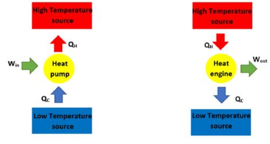
The second law of thermodynamics stipulates that 100% of work can be converted to thermal energy through heat transfer but it is impossible for 100% of thermal energy to be converted back to work due to inherent irreversibilities in nature arising from the randomness of particle motion and the tendency to diffuse or spread out over time. Heat naturally flows in the direction of decreasing temperature in nature, from hot to cold. The best we can theoretically get is a fully reversible process that gives back exactly what it takes from the Multiverse. In such a case, entropy is preserved at zero (it does not change during a full cycle + reversal). Any attempt to convert less useful thermal energy into useful work involves a machine called a heat engine. Heat engines are commonly found in car engines or coal powerplants. Their operating principle is to receive heat from a higher temperature source, apply a mechanical mechanism of harnessing part of the heat transfer, then dumping the rest of the wasted heat transfer to a lower temperature sink (normally the surrounding environment). The mediation of heat transfer is done by a working fluid, usually a coolant running through pipes. A heat engine must receive thermal energy from a hot source and dump thermal energy to a cold sink in order to do work: to receive and dump thermal energy via heat transfer from only a single reservoir is impossible to do work as thermal energy must be dumped to create a temperature differential to continue the cycle. Heaters work in the opposite principle, where 100% of work (electricity) is converted to thermal energy through heat transfer. For heat engines, the actual efficiency is given by E$_{actual}$ = 1 – (Q$_L$ / Q$_H$) where Q${}_L$ and Q${}_H$ are measured (actual) values of heat rejected to the cold sink and heat absorbed from the hot source, respectively in Joules. If we wish to know what the theoretical maximum upper efficiency can be for any process with a temperature differential between a cold and hot source, we can construct an idealized reversible heat engine called a Carnot engine.

This engine will set the theoretical maximum efficiency possible. In the real world, nothing can ever be higher than Carnot efficiency. The efficiency of a Carnot heat engine is given by E$_{Carnot}$= 1 – (T$_L$ / T$_H$), where instead of heat transfer we measure the absolute temperature (in degrees Kelvin) difference, since Carnot heat engines are reversible and there are no irreversible losses via heat transfer. For an ordinary combustion engine of a vehicle, the cold sink is the coolant in the radiator where an engine dumps its thermal energy via heat transfer operating at around 100 degrees (373K), while the hot source is the combustion chamber operating at around 900 degrees (1173K) therefore the maximum efficiency of a combustion engine is 1 – (373/1173) = 68%. The result is theoretical but nevertheless demonstrates the challenge of efficiency due to entropy. Actual efficiencies of combustion engines are normally in the range of 20-35% due to irreversible heat transfer and other energy losses. Modern engineering designs increase efficiency only marginally. When heat flows in the direction of increasing temperature, from cold to hot, it does not happen spontaneously in nature – it requires work. Such devices are called heat pumps. Refrigerators and air conditioners are heat pumps that remove thermal energy from an environment in need of cooling and dump it via heat transfer to a hotter environment using electrical work (usually the outside environment). A compressor does the bulk of the work, so when an air conditioning or refrigeration compressor fails, it is catastrophic to the entire unit. The cycle is contained within pipes where the working fluid is a coolant which contracts and is cooler than its surroundings thus allowing heat transfer away from the room or fridge to the coolant. A compressor does work on the coolant which then expands to gas form and moves closer to the hot sink, where it is hotter than its surroundings thus losing thermal energy via heat transfer to the surrounding air, with the aid of fans. After dumping thermal energy via heat transfer to the hot sink, the working fluid condenses and the cycle repeats. Throughout the process, energy is lost due to entropy through irreversible losses via the pipes. The compressor does work against the natural entropic flow of the Multiverse to cool down space.

Energy’s Lesser Known Brother: Exergy

Let us define the concept of exergy. The concept is useful not only for engineers prospecting a mineral deposit but for macroeconomic resource management in geopolitical analysis. If a mineral deposit or economy is assigned a total energy capacity, that is, the energy stored within its defined boundaries, then it is safe to assume some of that will be wasted during conversion processes. We are thus left with exergy – the work potential or available energy to do work. Exergy is therefore a fraction of the total energy, from irreversible losses due to entropy. A system is a dead state when it is in equilibrium with its surroundings. Such a system cannot do useful work as there are no gradients or differentials in temperature, pressure, velocity, height or chemical reactivity. We must make the distinction here between the boundary of surroundings: immediate surroundings and wider surroundings. The immediate surroundings refer to the portion of the wider surroundings in direct contact with a system and its processes, say chemical reactivity or heat transfer. The wider surroundings are the rest of the environment that is on aggregate, unaffected by the system and its processes. When a thermodynamic process exhausts itself and goes to a dead state at the end of a process, in equilibrium with its environment, it maximizes its work potential or exergy. If however, the temperature in its final state is different from that of the environment, or its pressure or velocity are different and not equal from those of the environment, then we can always generate work by running a heat engine or turbine through it to harness surplus exergy. Once the system reaches a dead state, there is no more work potential to be harnessed, as the energy required to move it into a non-dead state will be greater than any benefit extracted, unless that initial energy input sets it into a transient spontaneous cyclical motion during which we can spontaneously harness exergy from gradients and differentials. The atmosphere is commonly regarded as a dead state on aggregate, since it is used so often as the reference point i.e. the surrounding environment itself. The atmosphere has a tremendous amount of energy but no ability to do any useful work with it (zero exergy). Exergy can be harnessed locally through wind turbines for example, but strong directional winds are a less entropic and more useful form of energy than random and chaotic whirlwinds, which dominate the overall atmosphere. The greater the gap between energy and exergy for a system, the more room for improvement exists in engineering better efficiencies.

Solids & Liquids

For solids and liquids, we usually assume a constant average specific heat capacity (C$_{av}$) which scales linearly with mass. These values are found in tables for various substances. They refer to the readiness of a substance’s capacity to absorb thermal energy.

For all reversible, isothermal (constant temperature T) processes on the other hand, change in entropy can be defined as

ΔS = ΔQ/T

At high T, many states are already occupied; adding energy opens proportionally fewer new ones. If temperature is how full a hotel is, heat transfer would be new guests arriving. An empty hotel (low temperature) with 10 new guests sees a large change in occupancy, with lots of new arrangements possible. A near-full hotel (high temperature) with 10 new guests must squeeze them into fewer arrangements. The entropy, or “impact per guest” is therefore inversely proportional to how full the hotel already is. Division by T weights each Joule by its “disorder impact,” which decreases as the system gets hotter. The logarithmic form reflects that doubling the temperature doesn’t double the entropy. Each temperature interval contributes proportionally less as T grows.

Many 19th century physicists were pondering the ideas that would eventually make up the study of thermodynamics, in the wake of the industrial revolutions. There was James Watt, Sadie Carnot, Ludwig Boltzmann, William Thomson (Lord Kelvin) and Rudolph Clausius, to name a few. At the crux of it stood not only the challenge of capturing and formulating the relation between heat transfer and temperature but understanding the difference between reversible and irreversible processes and why differences exist. These differences would give rise to the notion of entropy itself. Heat transfer and work are merely forms of energy, therefore they are path-dependent. James Watt showed the equivalence between heat transfer and work, how a unit increase in the temperature of water could be brought about either through work or heat transfer. However the directionality mattered if the process was irreversible: 100% of work can be converted to heat transfer but 100% of heat transfer can never be transformed to work. Sadie Carnot showed the maximum possible theoretical efficiencies that were attainable for engines, given these constraints. Lord Kelvin established a temperature scale that began at the lowest temperature attainable in the entire Multiverse, “Absolute Zero”, at 0 Kelvin (-273C). Note that this implies 0C is 273K: or in general Kelvin units = Celsius units + 273. As the groundwork for thermodynamics was being laid, Rudolph Celsius formulated his famous inequality that explored the relation between heat transfer and temperature. Heat transfer is a form of energy, mostly thermal energy. Higher values of heat transfer have molecules with higher thermal energy – their kinetic energies and distances between them increases, as do the number of possible configurable states. Temperature is proportional to thermal energy but temperature is not a path-dependent property like heat transfer, it is state-dependent. This means it does not matter what path temperature takes, what matters is the initial and final states and the difference between them. A path-dependent property cannot simply be calculated by the relative difference between start and end state. In addition to temperature and entropy, volume and internal energy are state-dependent properties. A 1kg of boiling (100C or 373K) pan of water can either get to that state by heating it from a lower temperature (e.g. 70C) by mechanical work or by cooling it from a higher temperature (e.g. 130C) by pure heat transfer and zero work. Let us assume the same energy via heat transfer is applied to both scenarios and that the specific heat capacity (C${}_{av}$) of 1kg of water at 100C is 4186J/Kg⋅K. In the first scenario, Q = m×C${}_{av}$×(T$_{final}$ – T$_{initial}$) = 1×4186×30C = 125580J of energy is added while the second scenario removes Q = m×C${}_{av}$×(T${}_{final}$ – T${}_{initial}$) = 1×4186×-30C = -125580J of energy. The entropy change in the first scenario is given by ΔS = C$_{av}$⋅log$_e$(T$_2$ /T$_1$) = 4186⋅log${}_e$(373/343) = 351J/K but in the second scenario it is ΔS = C${}_{av}$⋅log${}_e$${}_{}$(T${}_2$ /T${}_1$) = 4186⋅log${}_e$(373/403) = -323.8J/K. The notable lesson here is that there is a scaling between temperature differences according to a logarithmic curve such that a colder system has more potential for entropy increase than a hotter system. The same energy and temperature difference has a bigger impact on entropy in the second scenario: each joule of energy begets more entropy. In the second scenario molecules have thermal motion already at 130C or 403K, removing energy constrains their motion and lessens their configurable states. In the first scenario, molecules have lower thermal motion at 70C or 343K, adding energy liberates their motion and raises their configurable states. In the end, both scenarios land on the same final temperature (373K) with the same net amount of energy (125580J) applied to both. Ignoring the sign differences and focusing instead on absolute values, the 125580J in energy increases entropy more for the water in the first scenario because the path began at a lower temperature, and this is the key takeaway. For most people, the assumption that higher heat transfer is linearly proportional to temperature makes sense but it misses the subtlety in non-linear gradient between each unit of energy and relative temperature changes, which is essentially what entropy is measuring. This is why we divide heat by temperature to get entropy and not multiply them together which would be a purely proportional relationship. If adding water to a container is like heat transfer, then the dimensions of the container would be temperature. Entropy scales with energy at different temperatures in non-linear fashion. Adding thermal energy via heat transfer to a cold system changes its entropy more than adding the same heat to a hot system.

Entropy is influenced only by temperature changes, as volume is fairly steady and pressure has very little impact, similar to incompressible gases. For compressible gases, in addition temperature, entropy is influenced significantly by pressure and volume. If we consider heating 1kg of water from 20C (T1 = 293K) to 100C (T2 = 373K), with a specific heat capacity of 4186J/Kg⋅K, the change in entropy is given by doing the proper integral, substituting Q as a function of T and summing all contributions of Q varying with T according to the natural logarithm:

ΔS = m×C${}_{av}$×log${}_e$(T${}_2$/T${}_1$) = 1×4186×log${}_e$(373/293) = 1010.5J/K

Alternatively, if we take the mid-point of 20C and 100C (60C or 333K) as a constant temperature for the system, the integration can be ignored

ΔS = ΔQ/T = m×C${}_{av}$×ΔT/T = 1×4186×(373-293)/333 = 1006J/K

For reversible processes, the change in entropy for a closed integral is 0: for irreversible processes, the change in entropy is always negative. At 100K a 100J boost of energy provides a Q/T = 100/100 = 1J/K entropy change. At 1000K, a 100J boost of energy gets much less mileage in entropy, Q/T = 100/1000 = 0.1J/K. This is because at the higher temperature, the configurable states and randomness of sum-parts are already high and 100J provides merely a marginal increase. A fully reversible Carnot heat engine operating between a hot reservoir of T${}_H$ = 600K and cold reservoir of T$_C$ = 300K has a Carnot efficiency of E$_{carnot}$ = 1 – (T$_L$ / T$_H$) = 50%, with Q$_H$ = 600J of heat absorbed from the hot reservoir where 300J is dumped into the cold reservoir and 300J goes into mechanical work, with zero losses. Here the change in entropy is given by a closed integral consisting of two sub-processes – heat transfer across the boundaries of the hot and cold reservoirs: ΔS = δQ/T ​= Q$_H$/T$_H$ + Q$_C$/T$_C$ = 600/600 + -300/300 = 1-1 = 0. The change in entropy for a pure reversible process is 0. A realistic engine with irreversible losses captures those losses in the following way: the change in entropy would see more heat dumped to the cold reservoir (Q${}_C$ = 350K) and less energy available for useful work (W = 600K – 350K = 250K) and so ΔS = δQ/T ​= Q${}_H$/T${}_H$ + Q${}_C$/T${}_C$ = 600/600 + -350/300 = -0.167J/K, which as expected is negative. The irreversible losses generated are represented by the change in entropy of -0.167J/K. Finally, the equations can even be used to test the validity of engineering claims. A manufacturer claims a refrigerator can transfer 400J from a cold reservoir TC = 250K to a hot reservoir TH = 350K with 50J of work, i.e. 450J is transferred to the hot reservoir. Is this feasible? The Clausius Inequality of the refrigerator is given by δQ/T ​= Q${}_H$/T${}_H$ + Q${}_C$/T${}_C$ = -450/350 + 400/250 = 0.314 which is impossible, as it is positive. Either the claims of heat transfer need to reverse (400J from the hot reservoir instead) or more work needs to be done (e.g. 350J) for this refrigerator to operate in the real world.

Gases

It is worth going over the basics of gases in order to understand the two conflicting worldviews that thermodynamics was grappling with during the 19th century. In physics, most gases are governed by the Ideal Gas Law, PV = nRT, a formula that brings together the most salient state-dependent properties of gases: pressure (P), volume (V), temperature (T) and number of molecules (n). Gas properties were studied by physicists much earlier but it wasn’t until the 19th century that French and Russian chemists unified previous observations made by Boyle, Charles and Avogadro. They noted that for many gases irrespective of substance, volume was inversely proportional to pressure when temperature was held constant (V∝1/P), volume was proportional to temperature when pressure was held constant (V∝T) and volume was proportional to number of molecules when temperature and pressure were held constant (V∝n). Amedeo Avogadro derived Avogadro’s Constant, a compact measured approximation for the number of particles in substances, defined by the unit of moles where 1 mole contains 6.022×10$^{23}$ particles (molecules, ions, atoms). He also hypothesized that equal volumes of gases at the same temperature and pressure contained equal number of particles. Putting together all three properties into equation form and replacing the proportionality sign with an arbitrary constant (i.e. V = R$_1$/P, V = R$_2$T & V = R$_3$n), each gas had its own equation of form VP = nRT where R is an arbitrary constant specific to the gas in question. Avogadro then plotted the charts of each gas and derived a universal constant when pressure was zero, calling it the universal gas constant (R), a constant in nature which arbitrates in units of energy per mol⋅Kelvin, the same dimension of the value VP/nT. The universal gas constant equals 8.314J/mol⋅K, for all gases. Volume multiplied by pressure in the numerator is energy in Joules, or unit of force conveyed per meter (Newton meters). The Ideal Gas Law explains what happens at the macroscopic picture when ensembles of particles are aggregated by state-dependent properties such as T, P and V. But at the microscopic picture, another equation emerges, the total energy of the gas or PV equals the sum of all the kinetic energy of individual particles. If the total energy of the gas is assumed to be 100% kinetic energy, the energy of 1 particle is 0.5mv$^2$ assuming all equal weighted particles and velocities in all 3 dimensions are equal, PV = 0.5mv$^2$×N for N particles. However, pressure acts only in 1 dimension perpendicular to the container wall leaving the other 2 dimensions irrelevant but each particle rebounds off the wall carrying twice the energy so the expression is scaled by a factor of 2/3: PV = 0.5mv${}^2$N×(2/3) giving PV = 1/3×mv${}^2$N. As a result, the ideal gas law has two versions, the macroscopic (PV = nRT) and microscopic (PV = 1/3×mv${}^2$×N). A physicist named Ludwig Boltzmann equated both

nRT = 1/3×mv${}^2$×N

The number of moles of substance, n, is given by N/6.022×10$^{23}$ therefore the N cancels out, leaving a constant fraction on the left equal to the universal gas constant (8.314) divided by Avogadro’s constant (6.022×10${}^{23}$). This gives rise to a new gas constant, k$_B$ = 1.38×10$^{-23}$J/K that arbitrates on a per molecule basis rather than on a per mole basis, thus bridging the macroscopic and microscopic worlds in thermodynamics. The resulting constant was named Boltzmann’s constant (k${}_B$). At room temperature (T = 300K) the average energy per particle is the Boltzmann constant multiplied by 300 to give ~ 4.14×10-$^{-21}$J. Temperature is akin to the average kinetic energy of particles and kinetic energy has components in all 3 dimensions. Purely orthogonal movements to the vertical axis are deemed kinetic energies while any motion parallel to the vertical axis in line with gravity is potential energy. Thermal energy is generally the sum total of kinetic, potential and internal energies of all particles.

Entropy Is In The Eye Of The Beholder

Computing entropy at the microscopic scale can utilize the Boltzmann formula for entropy, S= k$_B$⋅​ln(W), giving rise to a statistical mechanics perspective on entropy. The formula computes the entropy at any given time for a state, it does not compute changes in entropy over time. The critical variable is W, the number of possible configurable states in a system. When probabilities are used to capture microscopic configurations, the formula is called the Gibbs formula for entropy, S= -k${}_B$∑p$_i$⋅​log$_e$(p${}_i$). The microscopic formulae for entropy captures thermodynamic disorder. For small systems with limited configurations the calculation is simple. But for systems with more moving parts, it becomes a complex combinatorics problem. There are many types of entropy formulas to suit various granularities. Information theory uses the Shannon formula for entropy, S = -∑p${}_i$⋅log$_X$(p${}_i$) where the choice in base logarithm, log$_{X}$, defines the resulting units of entropy (x= 2 or log$_2$ gives “bits” while x= e or log$_e$ (ln) gives “nats”). The information theoretic formula for entropy captures information uncertainty.

Let us now illustrate the various entropy formulas with an example. Suppose we have a microscopic system consisting of 3 electrons each with possible spin states of only up (“U”) or down (“D”) when measured at the point of wavefunction collapse (they must be assumed to be superpositions of both states when unmeasured according to quantum theory). Spin states can repeat and ordering does not matter. What would maximum entropy look like? What would minimal entropy look like? And what would an intermediate state look like? When you have n things to select (spin states) while selecting m of them (electrons) at any given time, we have n$^m$ possible permutations, 2$^3$ = 8 in this case: UUU, UUD, UDU, UDD, DUU, DUD, DDU & DDD. There are 8 microstates with 1/8 probability, meaning this is its most granular configuration space. But entropy is not a fixed intrinsic property of any system, its value depends on the measurement. If we begin to coalesce microstates into macrostates, we lose some information in the process and probabilities change. If the macrostates are defined by the number of up spins, there is 1 macrostate with 3 up (UUU) with 1/8 probability, 3 macrostates with 2 up (UUD, UDU, DUU) with 3/8 probability, 3 macrostates with 1 up (UDD, DUD, DDU) with 3/8 probability and 1 macrostate with 0 up (DDD) with 1/8 probability. Contrast this to the maximum entropy state of all microstates each having 1/8 probability.

Remembering that we have probabilities, the Gibbs and Shannon entropy formulas can be applied to calculate the total static entropy of the system at a given time:

8 microstates (maximum entropy state):
Gibbs Entropy: S = -k${}_B$∑p${}_i$⋅​log${}_e$(p${}_i$) = -1.38×10$^{-23}$ ×[8 ×(1/8 ×log${}_e$(1/8))] = 2.86 × 10⁻²³ J/K
Shannon Entropy: S = -∑p${}_i$⋅logX(p${}_i$) = -[8 × (1/8 ×log₂(1/8))] = log₂(8) = 3bits

4 macrostates (lower entropy state):
Gibbs Entropy: S = -k${}_B$∑p${}_i$⋅​log${}_e$(p${}_i$) = -1.38×10${}^{-23}$ ×[1/8× log${}_e$(1/8) + 3/8×log${}_e$(3/8) + 3/8×log${}_e$(3/8) + 1/8×log${}_e$(1/8)] = 1.733 × 10⁻²³ J/K
Shannon Entropy: S = -∑p${}_i$⋅logX(p${}_i$) = -[1/8×log₂(1/8) + 3/8×log₂(3/8) + 3/8×log₂(3/8) + 1/8×log₂(1/8)] = 1.81bits

As is evident, maximum entropy (pure disorder) occurs at the maximal microstate configuration space of equilibrium where all states are equally likely. Minimal entropy (pure order) would be defined by a state where no distinction is made between macrostate and microstate. Entropy equal to 0 would occur when there is only 1 state (the logarithm of 1 equals 0) with all other states having a probability of 0. When we arbitrarily introduce macrostates by lumping together microstate probabilities (e.g. all electrons with up spins), this highlights a fundamental principle of entropy: coarse-graining, which is the process of arbitrarily aggregating microstates into macrostates. Coarse-graining is common in molecular chemistry where drug design is governed by computational molecular design. Using highly granular representations of molecules may be true to their original forms, but presents computational challenges when folding and simulating bonding sites, therefore molecules are rolled up into macro-molecules with a smaller set of active bonding sites to reduce simulation cycles. While entropy decreases and information is lost in the lower resolution designs, lesser degrees of freedom speed up discovery. Within a macrostate there can be many microstates. Entropy attempts to encapsulate the energy interplay between microstates and macrostates per unit temperature, where an increase in 1J/K in entropy represents the corresponding dispersion of molecular energy that contributes to disorder and increases its unavailability for useful work due to inherent irreversibilities. Over time, the total entropy of the universe increases, and the portion of energy that can be converted into work decreases. Higher entropy not only means more dispersion but is also correlated with more microstate permutations. A unit of energy in a system already flush with low quality energy and high randomness has less mileage for useful work potential than in a system defined by high quality energy and less randomness. If the microstate is identical to a macrostate, entropy change would be zero. Entropy only arises when gradients exist and there is micro-macro state “mixing”. In the example above, as we went from 8 microstates to 4 macrostates, the Gibbs entropy decreased by (2.86-1.733) × 10⁻²³ J/K = 1.127 × 10⁻²³ J/K while Shannon entropy decreased by (3-1.81) = 1.19 bits. The different units show the entropy of mixing, how 1.19 bits of information were lost when microstates were rolled up into macrostates, losing some grain while the 1.127 × 10⁻²³ J/K units in entropy lost, consistent with the Boltzmann constant, can be thought of as the “energy per unit temperature” in space and time that is no longer available for useful work.

Entropy Is All Around

The theoretical limit of Absolute Zero in a “heat death of the Multiverse” scenario, when not only average temperature fluctuations finally hit their physically lowest limits possible (~-273C), but the Multiverse is almost perfectly uniform in density. Matter would no longer exist in any macrostate such as galaxies, planets or even atoms. The Multiverse will go back to being pure microstates of subatomic wavepackets, just as in its early infancy. There would be no longer any distinction between past, present and future, the ultimate maximum entropy state. Another application of entropy is in large language models (LLMs), when a “loss function”, L$_{LOSS}$ = -log$_e$[p(x)], computes the entropy for predicted tokens during backpropagation to assess how well the prediction of the next token p(x) is compared to the actual token. The worse the prediction, the lower the probability and higher the entropy value. The logarithm of a higher value is used as a clever hack to penalize wrong predictions so gradient descent is adjusted in a slightly more likely manner during the next iteration. Language too, has evolved over time towards greater entropy due to the higher complexity and dimensionality that arises from ever-nuanced expression and abstraction. The progression from Cuneiform to modern digital language has seen a global entropic increase in line with the second law of thermodynamics, but also localized bubbles of order within the overall trend, such as great works of literature, film and art which are compact and low entropy manifestations of language.

The entropy of structural grammar and syntax in language may stay relatively constant over time. But if we think about how many more metaphors have emerged over time to enable deeper expression with language, coupled with the growing number of analogies, the evolution of language is humanity’s evolution of ideas. Measuring how entropy of content has shifted per message is a difficult academic question to answer, on the surface of it, quite ambiguous. Is language plagued with less expression available for meaningful content (higher entropy) or has it earned more expressive power (lower entropy)? The much overlooked philosophical work of Jaques Derrida’s Deconstructionism raises very important questions on the limitations of expression through language. According to Derrida, the core challenge in understanding the world through language lies in the gap between “signifiers” (words or symbols) and “signified” (meanings). When two people are exchanging ideas with a common tongue, the agreed-upon words they exchange (signifiers) can mean very different things to each person (signified). This gap is not just a matter of translation but also reflects deeper structural issues within language, as meanings evolve over time and across different cultures. Derrida dismantles barriers between signifiers and signified by questioning fixed meanings, in a sort of theory of relativity for language. In terms of entropy, if the uncertainty in conveyed meaning with language was indeed in accordance with Deconstructionist interpretations, language would be far more entropic than otherwise assumed. Metaphor and analogy have proliferated in many domains, pushing up the expressive richness per unit of content, which can be viewed as a decrease in entropy if messages encode more meaning with less ambiguity. But it could paradoxically increase entropy if content becomes more noisy, or context-dependent. Information overload and media complexes that prioritize superficiality and emotion over depth and reason would render language more entropic. The evolution of culture and society plays a crucial role: if standards are falling, vocabularies are becoming cruder and average intelligence is faltering, entropy in language would fall to a lower state, which on the upside, would allow society a windfall potential for future expressive capability out of said retrogression. Generative AI can reduce uncertainty for the user in some contexts, while AI-synthesized content can increase informational noise elsewhere, increasing language entropy. The proliferation of AI “slop” is one such manifestation.

Data compression is another great example of information entropy where entropy is reduced by removing redundancy from language. For example, in a message with 1000 characters containing 10 identical blocks of the string “1000000”, the string can be encoding with “0” instead, reducing 70 characters but adding 10, giving a net reduction of 60 characters. The entropy of the original message was 1000 characters but a net 60 were removed, 6% reduction in entropy. This is the information that is now freely available for useful work such as adding extra information to the message. Data compression in text, image, audio and video can reveal how much redundancy exists in information. Highly predictable information with redundancy compresses well, while unpredictable or creative information does not compress well, retaining a higher entropy. Standard compression algorithms are lossless, meaning information is generally not lost, absent some random codec errors. Lossy compression on the other hand, common with audio and video, trades some information loss for speed, resulting in some irreversible distortion of the source material. Lossless compression is generally reversible while lossy compression is irreversible. Ergo, the entropy lost with lossy compression can be partially offset by some irreversibilities. In audio for example, sounds beneath 20Hz or above 20kHz, typically inaudible for average adults, can be truncated in lossy compression. This is information permanently lost in translation. Generally, if an information domain is predictable and repeatable (e.g. legal corpora), the potential for compression and entropy reduction is far greater. Data science is yet another fascinating example to think about information entropy. A dataset at its most granular level of grouping and aggregation, financial data for example at the tick (second) level, would form the baseline “microstate”. The baseline microstate would see a higher noise-to-signal ratio than weekly level of aggregation, and would constitute maximum entropy in terms of near-uniform probability of each next discrete step interval (the following second), of price moving up or down. If the data however, was rolled up into macrostates of hourly, daily or weekly intervals, then some information about the price is inevitably lost and greater signal than noise will emerge, allowing trends and seasonality to be extracted – higher quality information. This is why entropy would decrease and a higher order would emerge in macrostates relative to the microstate.

Modelling Geopolitics In An Entropic Framework

Geopolitics, sociology, psychology and economics are not pure sciences as their core subject is human beings, who do not behave rationally especially when masses of individuals come together and group psychology begins to dominate social dynamics. Individual humans can be very difficult to model, – they are complex and unpredictable. Without an empathic understanding of their personal journeys, information asymmetry masks true motivations. However, when masses of individuals come together to form societies and economies, their collective behavior can become much more predictable. As such, statistical mechanics and probabilistic models will work much better with aggregates. There are parallels with quantum mechanics and human societies. Individual atoms are chaotic and defined by randomness, but masses of atoms are more easily predicted through statistical and probabilistic frameworks. Entropy is non-linearly bound with temperature by logarithmic scaling, the higher the starting temperature in a system, the lower the entropy for the same amount of energy put into the system than a colder starting temperature. Adding thermal energy via heat transfer to ice at -1C will melt the structure, but the same energy added to the surface of the sun will not even dent entropy. A geopolitical system with high institutional trust and cooperative density will absorb a crisis with minimal entropy cost, while a system with low institutional trust and cooperative density will suffer a catastrophic entropic explosion from an identical crisis. The more one ponders man-made constructs, one inevitably realizes that we too are at the mercy of entropy as much as nature: why not apply the principles to model geopolitical macrosystems? What I am going to propose is not a rigorous statistical model of reality, this is merely a conceptual framework to help the reader connect the dots, and perhaps motivate the more technical savvy among us, to go one step further and devise a testable model using this framework. Note that this is a static entropic framework which computes system entropy change between 2 static states, it does not model the time evolution of system entropy (Kolmogorov-Sinai entropy), which would be out of scope of this article and difficult to apply. The framework will calculate entropy of a geopolitical framework at any given state (static). The values on their own are meaningless. It is only when entropy differences between an initial and final state are computed, does it become meaningful with regards to the direction of a system’s evolution. It may be helpful to do this across multiple possible states as well, comparing state entropy changes laterally. Taking the difference between 2 global states across time would be equal to the change (rise or fall), in geopolitical uncertainty. Begin with the initial state (e.g. at t = 0) and a final state (e.g. at t = 1), calculate each value of S$_{geo}$ and compare the changes. Which path creates more or less entropy?

The Entropy Model

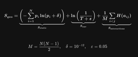
where:

The central insight of the framework is that the destruction of cooperative institutions generates more uncertainty than the redistribution of power (S$_{env}$ >> S$_{static}$). The same crisis costs far more entropy at T = 0.10 than at T = 0.90. A geopolitical system at T = 90 (high trust) can absorb the same crisis with minimal entropy cost. A system at T = 10 (low trust) suffers catastrophic entropic collapse. The variable T is akin to the heat capacity of the international order. The Religious Zionist Fascist machinery under Trump and Netanyahu embody this observation in the real world today. Coupled with centuries of Anglo-American perfidy and duplicity, fake negotiations rooted in ill-will and a shameless, remorseless Religious Zionist disregard for any soft power, a rapidly rising entropy is being served upon the globe. How quickly each term’s contribution to overall entropy moves depends on events but generally the S${}_{static}$ term will move slowest. All three terms are independent reservoirs of uncertainty, which is why they are summed. The environment entropy term, S$_{env}$ is the driving force, akin to the “temperature” of the global environment, which modulates everything else. Entropy signifies uncertainty about which configuration the system will occupy next. It is not strictly “disorder” or “chaos” and not a moral judgment. Empires create low entropy environments due to higher predictability and mono-culture. Imperial collapses create high entropy environments due to lower predictability and multi-culture. Higher entropy is not necessarily bad (think multipolarity and waning nefarious hegemony) while low entropy is not necessarily good (think of the pervasive Zionist Fascist influence post-USSR). Maximum entropy is not a world of enemies, it is a world of ambiguity. A system where all pairwise coefficients are 0.5 is a multipolar system where everybody is a frenemy – no permanent friends, only permanent interests. A system of two tight blocs (all pairwise coefficients are 1 within blocs and 0 across blocs) would give the last term, S$_{interactions}$ ~ 0, a world where relationships are perfectly predictable.

General guidance on model improvement: do not over-fit, if adding a new term to the equation, make sure it is not very cross-correlated with the other terms, otherwise it will merely add noise. Instead of arbitrary geopolitical numbering, using statistical indices to capture technological innovation, patent filings, annualized or rolling real PPP GDP growth, military power, net Current Account or public debt figures may add more objectivity. The framework is largely conceptual and attempts to replicate entropic principles from science onto geopolitics. Much depends on how accurate the arbitrary coefficients are assigned to represent the global dynamic, there is always room to improve here for those savvy enough with statistics and modelling.

Step 1: The Static Power Term (S$_{static}$). A subleading term which measures the uncertainty about which player holds power. A seasoned geopolitical analyst will fill out a N×1 matrix (table) between N players for each world state. The matrix will hold coefficients p${}_i$ between [1, 0] indicating their relative global power – the net sum of all contributing factors. A powerful country would constitute a higher value nearer to 1. The coefficients would be the relative weights and must be normalized and sum to 1 in order to complete the global power balance. These coefficients capture the established global power balance in the given state. Over time, they are the slowest moving term, forming longer term super-cycles and underlying geopolitical frameworks. The entropy of each player N is then computed and summed across all N players, not averaged since static power is a zero-sum game. A higher value of the static power term’s contribution to total geopolitical entropy (higher entropy) would correlate to a world where power is fragmented and decentralized across many players while a lower value (low entropy) would correlate to a world where power is concentrated across a few players. The entropy of each power node i is computed as -p$_i$${}_{}$⋅log$_e$(p${}_i$) (Shannon entropy) and summed for each world state. The delta term ẟ = 10$^{-12}$ is a hard floor to prevent errors in computing the logarithm of zero. It signifies a maximum floor entropy reduction of ~ -27.63 when a player has 0 power, but this is trivial since relevant players should always have non-zero coefficients.

We will build 3 hypothetical world state blocks representing a fading unipolar state (current era), a multipolar state (possible future state) and a consolidated unipolar state (e.g. the 1990s). Since entropy is not a path dependent property but a state variable, we only care about initial and final state entropies. We can thus use these states as building blocks in the model.

Step 2: The Environment Term (S$_{env}$). The the driving force of the model, – a leading term capturing the uncertainty generated by the collapse (or strengthening) in the global “temperature” (T) of its cooperative and diplomatic institutions which serve as the glue holding the world into a lower, more predictable entropic state. Wildcard shifts in global Zeitgeists such as the onsets of world wars, 1971 Nixon shock, 1979 Iranian revolution, 1991 fall of the USSR, 2001 Zionist-Wahhabi false flag attack, 2008 American financial crisis, 2016 reactionary movements in the Anglosphere (Brexit and Trump), 2022 NATO-Russia proxy war in Ukraine, all play pivotal swing moments i.e fast-moving temperature shifts. The temperature proxy T follows the same logarithmic curvature as the original form and is bounded between 1 and 0, with 1 being a fully predictable minimum entropy state when trustworthy diplomacy dominates, while nearer to 0 would indicate an environment marked by mistrust and conflict. The epsilon term ε floors the denominator such that it is never 0, which would present mathematical problems, and is fixed at a small value of 0.05. A higher value of the environment term’s contribution to total geopolitical entropy would correlate to a world where mistrust and conflict reigns while a lower value would correlate to a world where trust and cooperation reigns.

Step 3: The Interaction Term (S$_{interactions}$). A subleading term which measures the average uncertainty per bilateral relationship. A seasoned geopolitical analyst will fill out an [ N⋅(N-1)/2 × 2⋅W] matrix between N players and W world states. Each world state will hold bilateral coefficients between 1 and 0 per pair of players, capturing the relative attitudes between players, how accommodating they are to each other, and a column for the entropy value. In essence, a coefficient of 1 would signify ironclad allies, near 0 would signify sworn enemies, while 0.5 would straddle the “frenemy” zone. The coefficients are not constrained with summation, only that they be between 1 and 0. The coefficients capture the shifting dynamics beneath the slowly changing static geopolitical order. The entropy of each pair is then computed and averaged across all M = N×(N-1)/2 pairs. N = 8 players would give M = 28 pairs of values. The interaction terms are a finer grain than individual players, they are independent from the number of players N. This is why they are averaged. A high average value of the interaction term’s contribution to total geopolitical entropy would correlate to a world with a tangled web of ambiguous alignments while a low average value would correlate to clear blocs and predictable alliances. The entropy of each bilateral pairing is computed as H(a) = -a${}_i$${}_{}$⋅log${}_e$(a${}_i$) – (1-a${}_i$)⋅log${}_e$(1-a${}_i$) (Shannon entropy of a random variable). Ironclad allies are perfectly predictable, sworn enemies are also predictable but less so. The most uncertainty comes from “frenemy” relationships.

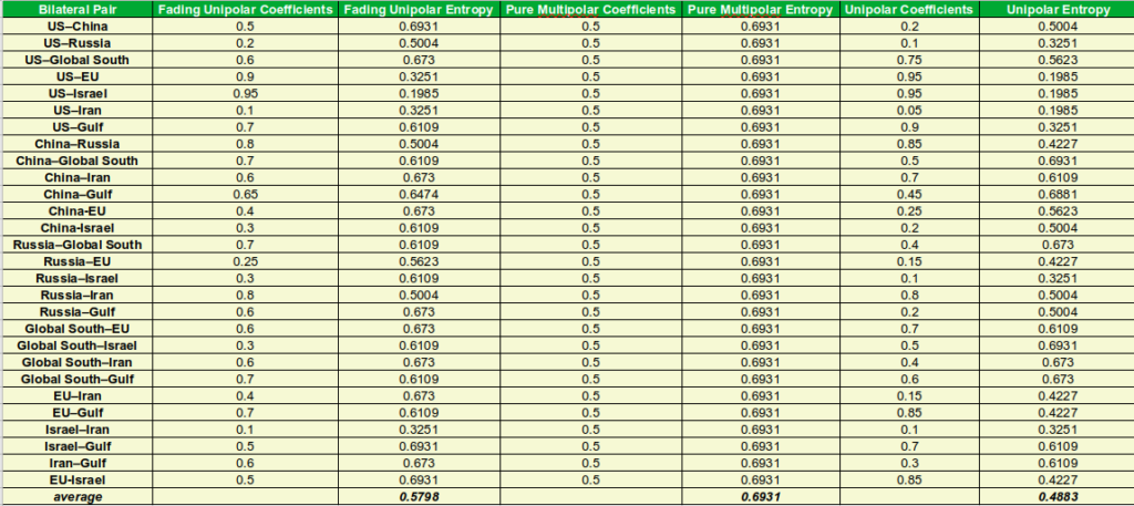
Now, for entropy calculations in a geopolitical context. Take each world state’s building blocks for each term and subtract them:

ΔS$_{geo}$ = ΔS${}_{static}$ + ΔS${}_{interactions}$ + ΔS${}_{env}$

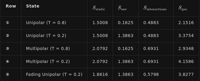
Transition 1: Unipolar -> Multipolar at Constant Temperature (T = 0.8)

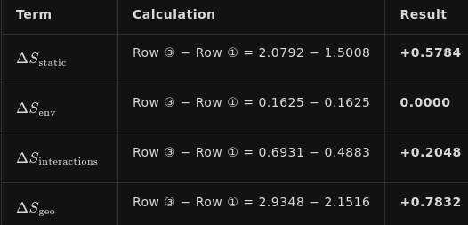
Transition 2: Unipolar -> Multipolar at Falling Temperature (T=0.8 to T=0.2)

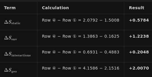
Transition 3: Fading Unipolar -> Multipolar at Constant Temperature (T=0.2)

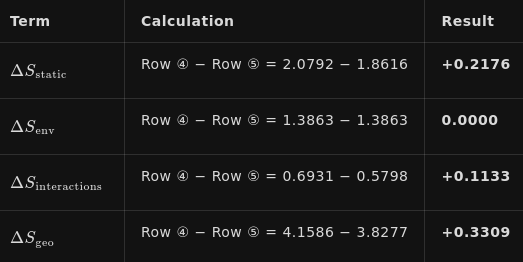
Transition 2 has the same structural transition as transition 1, but during a crisis (T=0.8 -> T=0.2). The environmental term now dominates: +1.2238 from the cooperation collapse. Total entropy is 2.56× higher because the system has no institutional heat capacity to absorb the shock. The T collapse in Transition 2 is the difference between +0.7832 and +2.0070. That extra +1.2238 is the environmental entropy released when institutions burn down during a hegemonic transition under shameless and remorseless Zionists like Trump and Netanyahu.

Which finally brings us to the main point in thermodynamics and its inherently terrifying beauty: The second law of thermodynamics applied to geopolitics.

The second law states that a process can decrease entropy locally but must increase, or at best stay constant, in the wider environment. If a globalized system of diplomacy and trade is destroyed by the malcontents of Anglo-Zionism, for example if T drops from 0.8 to 0.2 and system entropy S${}_{geo}$ increases by +2.78. We measure S${}_{geo}$ directly and infer the impact to the wider environment. We can never truly measure S$_{surroundings}$. By thermodynamics, in real irreversible processes, if ΔS${}_{geo}$​ is negative, we know someone, somewhere, burned enormous energy to make that happen. The local decrease is allowed but the surroundings pay the entropy cost. This is why building international order is hard and expensive,
while destroying it is easy. No external work needed. The system naturally slides toward higher entropy. But thermodynmaics gives no free lunches. All players pay the cost, as entropy in the wider global community is absorbed. Imperialism distributes ruination to the world, far greater than any improvements to the imperial core. Imperialism, through war and subjugation, distributes ruin and externalities onto weaker players, and weaker players are the global majority. While multipolarity according to the model produces higher entropy than hegemonic unipolarity, since empires are more stable and predictable, the key lies in T: in a world with a high T, the transition from Unipolar–> Multipolar increases entropy by less than a corresponding system with less T. However, the second law of thermodynamics in a geopolitical context merely sets the floor. The impact to the environment is at least equal to the entropy produced. Under a hegemonic system, it can be argued that ΔS${}_{surroundings}$ >> ΔS${}_{geo}$ while for a multipolar world with high T, ΔS${}_{surroundings}$ would not be much greater than ΔS${}_{geo}$.

Conclusion

Through the lens of thermodynamics, organic life is an entropy catalyst. Intelligent life goes one step further by accelerating global entropy according to the second law of thermodynamics, through locally decreasing entropy to create microcosms of order, such as literature, art, engineering feats, empires and civilizations amid a wider ocean of diffusion. On a long enough timeline, past, present and future will be indistinguishable from each other as their states will essentially fuse into one state with zero gradients. Entropy would be frozen at its maximum value, remaining constant and no longer increasing. Applying the Multiversal principles of entropy to a geopolitical framework has its merits in understanding the direction of global entropy, provided the users of the model understand its limitations.

Main Page